What do we want to do?

First things first, let’s start with what we wanted to do.

Generative models are trained on enormous piles of data, a lot of it copyrighted, and that has made one question suddenly quite pressing. It has been showing up in lawsuits from Getty against Stability to the major record labels against Suno and Udio: what does a model actually keep about what it was trained on?

There is a whole field, with many cool figures, trying to tackle this question: memorization. Importantly, there isn’t just one kind of memorization. The obvious one (and the main focus for now) is verbatim memorization, the model handing back a training image or a melody note for note, like this one from Carlini et al.. It is very impressive, but it is also rather rare, since it only happens to a handful of examples among tens of thousands. Instead of catching memorization at generation time, you can also look for it inside the model, where it takes a subtler form. A model can treat its training data differently from data it has never seen, reconstructing it a little more faithfully, behaving a little differently near it, following a trajectory a bit more specific to it, all without ever reproducing it.

Since “memorization” usually points to the verbatim kind, and to keep things clearly separated, we named this measurable asymmetry the membership signal: any trace you can read off a model that tells you whether a given sample was likely in its training set. Hence, it is not a fixed mathematical definition but rather a concept, anything that leaks information about whether a data point belonged to the training set.

To round out the context, there is an important point that is often misunderstood. What makes the broader memorization question, whether verbatim or the membership signal, so difficult is that you can train a model that has clearly absorbed a great deal of information from its training data while its loss curves still look perfectly healthy: no signs of overfitting, and a validation loss that decreases smoothly. There is seemingly nothing to see. So the whole point is: if this information does not show up in the loss curve, is there a place in the model’s behavior where it might be hiding?

A quick reminder on Flow Matching / Rectified Flow

Memorization phenomena are so subtle that techniques are usually tailored to a specific type of model: DDIM/DDPM, GANs, Flow Matching / Rectified Flows… Those last ones are the ones we focused on.

From now on I’ll just say Flow Matching for both Rectified Flow and Flow Matching. They are not eeexactly the same, but I’m quite sure it’ll be clear enough, and clearly less verbose. One other thing, here I am not talking about the Reflow procedure.

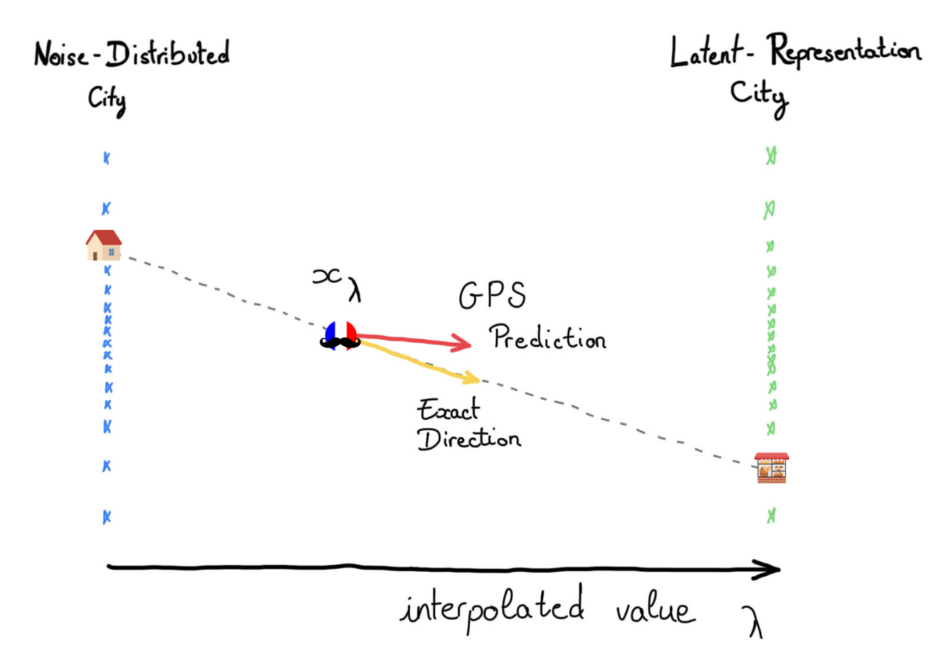
Before getting to the core, let me quickly recall the learning paradigm of Flow Matching. You are probably aware that It is a superstar (… even if its time may be coming, with one-step generation paradigms like MeanFlow or Shortcut models) behind systems like Stable Audio, FLUX, and Stable Diffusion 3. Here, we focus on the linear interpolation version. Pick a noise point \(x_0\) and a data point \(x_1\), draw the straight line between them, and a point on that line is \(x_\lambda = (1-\lambda) x_0 + \lambda x_1\). Here \(\lambda\) says how far along you are: \(\lambda = 0\) is pure noise, \(\lambda = 1\) is the data. The model’s whole job is to look at a point on this line and predict the direction that carries it toward the data. At generation time you start from noise and move along the path with small explicit Euler steps, and the model hands you the direction at each one.

Basically, imagine you are a Noise, at home (i.e. in your so-cosy Noise-Distributed City) and you want to go to your bakery (i.e. in Latent-Representation City, a very famous one) to buy a baguette (you are a French Noise). But your GPS only gives you the DIRECTION you should head in depending on where you are. So what you do is check the GPS, walk a bit, check the new direction, and so on. And this GPS didn’t come from nowhere: you and your Noise friends trained it beforehand by going from many places to many others, and each time, while on your way, you always fed it the straightest direction toward your destination.

Well, congratulations: if you were an extra-dimensional point, you just trained your own Flow Matching GPS using the linear interpolation path!

I actually did a whole blog post on RF / FM and the diffusion based generative paradigme, so make sure to check it if you need a reminder. ;)

Where did we look for information?

Finally (and I promise, after this we’re done with the setup), let me describe the probe itself.

Take one data point, from the training set or the held-out set, mix it linearly with noise to land at some position \(\lambda\) on the path, let the model predict the direction from there, take one big step, and reconstruct where it thinks the data should be. Compare that to the true point: the distance is the model’s error at that position. That is just the Flow Matching loss itself, read at a single \(\lambda\) instead of averaged over all of them:

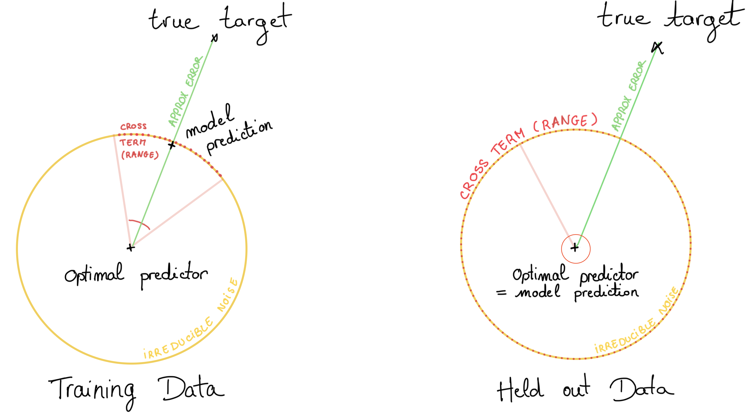
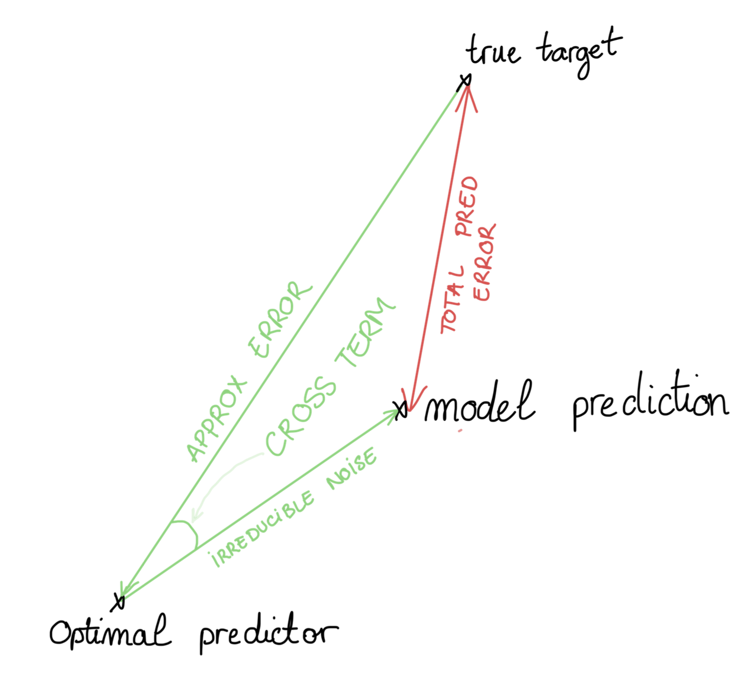
Now, it’s worth pausing on what this loss actually contains, because it’s the key to everything after. We decided to bring in the optimal predictor which is (obvisouly) the best any model could possibly do at this point. Expanding the squared norm gives three terms:

The first term is how far the model is from the best possible predictor. The second is the sample-specific residual, the part of the target that no predictor can infer from the current position alone. And the last one, the inner product which measures whether the model’s error is aligned with that residual.

The first two are, in a sense, “innocent”: every model pays them, on training and held-out data alike. The third one is the interesting one, and it’s the only place where being a member of the training set could leave a mark. (Keep it in mind, we’ll come back to it and make it fully precise near the end !)

So how do we get to it? The trick is a subtraction (what a trick!). We run the probe on many samples, separately for the training set and the held-out set, and look at the average difference in error between the two, as a function of where we started (i.e. the \(\lambda\)). Since the two “innocent” terms behave the same on seen and unseen data, they cancel out, and what survives is essentially that lonely cross-term, the one place a training bias could hide.

That those two terms behave the same on training and held-out data does rely on two mild assumptions, which describe a properly trained model:

Assumption 1 (Uniform approximation error). The model is no closer to the best predictor on its training points than on the population at large. In other words, it hasn’t done anything special on the samples it saw, which is what you get when the model hasn’t overfit in the classical sense (early stopping helps here). Note that this does not forbid a train-test gap in the loss; it only forces that gap to go through the cross-term.

Wait, doesn’t that assume the whole thing away? Not quite: the assumption fixes how far the model lands from the ideal prediction, the same for members and non-members, but says nothing about which way the leftover error points. That direction is where the leak hides, so we’re only ruling out crude memorization, not the subtle kind.

Assumption 2 (Representative sample). The empirical noise floor matches its true value, which is essentially just the law of large numbers for a large enough dataset.

And that’s the whole idea: the train-test gap is a subtraction designed to isolate the one thing we want, a bias (if it exists) toward the training data, el famoso membership signal.

The observation that started it all

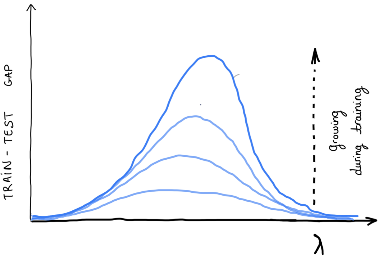
So now we had a clean setup and a way to measure this bias, but we genuinely didn’t know what it would look like. Maybe a flat line, if there’s no bias. Maybe a bump near \(\lambda = 1\), close to the data / noise or even both? Instead, in every single configuration we tried, the gap traced the same curve: a bell. Flat and near-zero at both ends of the path, rising to one clean peak somewhere in the middle.

It came back for audio and for images, for transformers and UNets, across latent spaces and noise parametrization. Obvisouly, it’s exactly what pushed us from “we have nice measurement” to “we need to explain why”. Why a bell at all, and Why does it peak in the middle?

Even crazier, this doesn’t appear randomly at the end of training. It grows steadily during training, well before any visible overfitting.

The Hourglass

Now that we’ve run through the experiments and laid out the setup, let’s get to the real explanations. Buckle up a little because there are several of them, they are all tangled together. But, in the end, they make a pretty nice story (backed up of course by theory and the experiments in the paper).

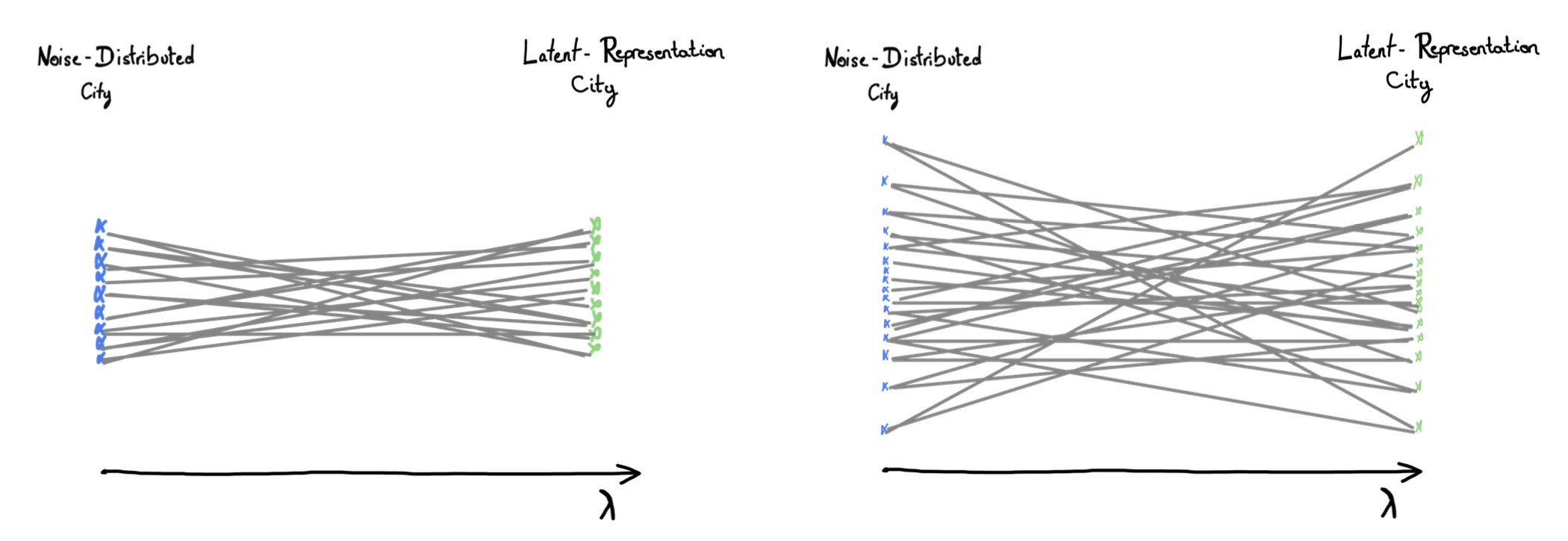
Let’s picture the Flow Matching path in 3D: two flat planes facing each other, the noise distribution on the left and the data distribution on the right, with the interpolation paths running between them. Every sample is a single straight line, tied from its noise point on the left to its data point on the right, so the whole thing is a bundle of straight spaghetti stretched across the gap.

Now pull the two clouds apart and look at the bundle from the side. Because each spaghetti strand joins a scattered noise point to a scattered data point, the bundle isn’t a uniform tube. It forms an hourglass: wide at both ends where the points are spread out, and pinched in the middle where all the spagheto funnel through a narrow waist.

And this bundle isn’t only a picture of the data. It’s essentially the flow field the model ends up learning: at each point in space, the spaghetti strands passing through are exactly what tell it which way to push. So the shape of the bundle is the shape of the model’s job, and what an interesting coincidence that the pinch of the hourglass seems to sit at the same place as the peak of the error, no?

Now think about the model’s job at each point: given your position, predict your direction. Near the ends, this is easy, and for the same reason at both. At the start, out in Noise-Distributed City, your exact position sits on essentially one sensible trip. You’re far from the bakery, the Latent-Representation City clustered off in one general direction, so where you stand points you cleanly toward where to go. And at the very end, near the data (i.e. your bakery), it’s the mirror image, you’re right next to your destination, only one trip realistically ends here, so again your position tells you your direction almost for free. Either way, few contradictory routes pass through where you’re standing, so a simple rule nails it.

In the mean time, in the middle your position sits in the crowded central square, the spot where trips coming from every home and heading to every specific places of Latent Representation City all cross. The same location is compatible with dozens of different directions, and no simple rule can tell which one is yours. Should I take this road or that one? Genuinely hard to say, and it’s exactly here that knowing a shortcut, or the specific one right answer, would save you the most.

Hence, there is a region on the path, where position becomes a much worse guide to direction because position alone becomes ambiguous. In the clean Gaussian case, we can even compute where that region sits in closed form, from the variances of the noise and the data alone, with nothing about the model in it. (We’ll come back to this later)

That’s the part I find most surprising. The peak is not just somewhere in the middle but rather its location seems to be fixed by the geometry of the problem. We change the architecture, the model size, or the training details, and the bell may get taller or flatter, but it stays in the same place depending on the data.

At this point, that’s only an observation and the theory will come later. But already suggests something a bit unusual: the model seems to impact how visible the leak becomes, while the data and noise distributions decide where along the path we should look for it. Even more, that stable location is also the region where the position is least helpful for deciding which direction to take.

Here, I’ve been a little sloppy on purpose. I suggested the model runs out of information, when what really runs out is one particular kind of it. Fixing that sloppiness is another really cool piece of the paper, so it deserves its own section.

Why the leak has to exist

Okay, as I just said, I lied a little (purely for pedagogical purposes, you know…). Near the pinch, the model doesn’t run out of all information, only the easiest kind to learn: the simple linear one, that “read your direction straight off your position” rule we just watched collapse in the crowded square.

One quick disambiguation, because linear is doing double duty here. The path is linear: the straight segment from noise to data, the spaghetti strands, and that never changes. What changes along the path is whether the direction can be read off your position by a simple linear rule. Two different “linears”, then: the road is always straight, but the guidance is only linear near the ends. It’s the second one that collapses at the pinch, and the leak lives in that collapse.

So what does nonlinear actually mean, back in the streets? A linear rule is a smooth one: shift your position a little and the right direction shifts a little too, in proportion. Step a bit east, aim a touch more west, nothing dramatic. That’s fine near the ends. But in the crowded square it breaks, because two spots barely a step apart can call for completely opposite directions: this walker peels off east toward the bakery, that one veers west toward the cinema, and they’re standing right next to each other. It is quite impossible for smooth, gentle rule to do that, and you need a rule that turns sharply depending on the fine details of exactly where you stand.

And notice why the smooth rule could never do the memorizing for us, however much data it saw. A linear rule is a single instruction that everyone follows the same way: “lean east in proportion to where you stand.” There is only one such rule for the whole city, so it has nowhere to store “you, specifically, third door on the left.” To single out one trip, the rule would have to change depending on which trip you are, and a rule that changes from spot to spot is exactly what we just called twisty. That’s not a coincidence: bending the rule to fit one trip is the definition of going nonlinear. So memorization doesn’t just happen to be easier in the nonlinear regime but rather can only live there.

This is where the distinction between generalization and memorization becomes a bit blurry. Near the pinch, the model cannot rely much on the simple linear rule anymore, so it has to learn more detailed turns. Some of those turns are genuinely useful: they point toward the right neighbourhood, and many trips share them. But the model never receives a clean label saying “this part is the neighbourhood rule” and “this part is just the turn toward this exact bakery”. It only sees complete trips. So the useful turn and the private detail arrive together. Across many trips, the shared part is what becomes generalization. But on any particular training trip, it is still mixed with small sample-specific quirks, and the model can absorb a little of those quirks while learning the useful structure.

This is roughly what I mean by a membership signal. It does not have to be a dramatic failure, or a memorized copy of the sample. It can simply be a small residue left by the fact that this exact trip was part of training. It’s the flip side of learning itself: to capture the real shape of the city, the model can’t avoid memorizing a few private doors along the way.

Why nothing shows up on the dashboard

So the signal is always there, we understand why it looks like this and why it has to appear. And yet no standard metric catches it. Why? There are two separate reasons that compound.

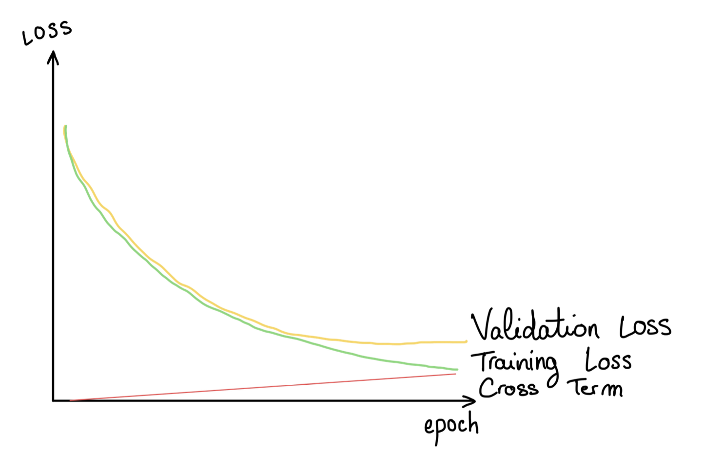
Dilution. The signal lives in a narrow band near the peak, but training monitors the loss averaged over the whole path. If you spread one sharp local effect across the entire interval, it barely moves the average.

Masking. This one is subtler. Early in training the model is still learning the generalizable structure, and that lowers both the training and the validation loss together. Underneath, on the training side, the leak term is quietly growing, but it is buried under the much larger gains from generalization. On the validation side, the leak term is absent, since the model never saw those sample-specific residuals. So validation keeps dropping and looks perfectly healthy, while the membership signal accumulates silently.

What the gap is actually measuring

A bit more explanation, but hang in there, we’re getting close to the end.

To understand what the gap is measuring, we need to come back to the decomposition I mentioned earlier. As I said Matching is trained with a mean squared error. If we insert the optimal predictor between the model prediction and the true target, the prediction error can be written as the squarred sum of two vectors: the model’s approximation error, and the irreducible residual, meaning the sample-specific part of the target that cannot be inferred from the current position alone.

Since the loss is the squared norm of that total error, expanding it gives two squared norms plus a cross-term that measures how aligned the two vectors are.

That alignment is where membership can appear. On held-out data, the model has never seen the residual attached to that point, so the alignment has no systematic direction and tends to average out. On training data, the model was fitted on those residuals, so a directional bias remains. The other two terms mostly behave similarly on seen and unseen points, so the train/held-out difference isolates this alignment term.

As you can see now, the gap is not just a convenient diagnostic but what’s left is the membership signal we were trying to isolate. And where along the path is it largest? If you didn’t skip straight to this line, you already know it is at the pinch of the hourglass.

From intuition to a real prediction

Everything so far has been intuition. To first need to turn it into something we can actually compute and verify. We will look at the one case where the maths stays clean: the Gaussian case.

In that setting, the optimal least-squares predictor is provably linear. So when we study the linear predictor, we are not just making a simplification but we are studying the target the network is trying to approximate in the ideal limit. And after some math, the membership signal turns out to be proportional to the irreducible variance (the part of the velocity that cannot be predicted from position).

That variance is largest exactly where the linear information vanishes, at the pinch of the hourglass. From that proportionality, the bell shape, the peak location, and the \(1/n\) decay all become much less mysterious. All those metaphors were pointing to something real, and the Gaussian case gives us a way to compute it.

Of course, a fair question is why a Gaussian model with an optimal least-squares predictor should say anything about a real transformer trained on real latents.

Well, it remains informative for two reasons. First, in the Gaussian case, the optimal solution is linear independently of the architecture used to approximate it so this what will tend to reproduce the transformer optimaly. And in practice, spectral bias suggests that neural networks tend to learn simple, low-complexity structure first, before fitting the more nonlinear scramble, which is exactly the part that becomes important when the linear signal weakens. Second, we work in the latent space of an autoencoder, and those latents are often designed to be roughly Gaussian and isotropic, either through an explicit KL penalty or through bounded activations like tanh.

So the Gaussian case is not meant to describe the world perfectly. It is the clean case where the mechanism becomes visible, computable, and therefore testable. In this context, we were able to derive a precise location of the gap’s macimum depending only of the Noise and Data covariance. Hence, the ultimate question is whether this actually happens in practice. (and it does ;) )

Does the whole story actually hold?

As we said, the nice thing about predicting a specific location is that you can actually try to break the prediction. So we tested it in both directions, this time directly with transformers and real latents.

First, we moved the peak on purpose. Our formula says that the location depends only on the covariances at the two ends of the path, so we pushed on each end. Scaling up the noise variance shifts the peak as predicted, and swapping the training dataset for one with a different structure shifts it again, with the prediction still matching.

Then we did the opposite and varied things that the theory says should not move the peak: the architecture (transformer versus UNet), the model size, and the sampling scheduler. The peak barely moved; mostly, it was the height that changed. Roughly speaking, the geometry of the data seems to decide where the peak sits, while model choices mostly decide how high it gets.

There is also a case where things become less clean. On image latents from a VAE, the distribution is much less Gaussian: heavier tails, stronger correlations, and generally a messier geometry. In that setting, the closed-form peak location failed. But the leak itself does not disappear. The gap is still there, with the same broad bell-shaped profile. So it is not that the Gaussian calculation invented the signal. It mostly gave us a clean way to locate it.

I find this more reassuring than disappointing. The theory is not magical, it gives a clean version of the mechanism under clean assumptions. When those assumptions become shaky, the exact location becomes harder to predict, but the broader picture remains: the signal concentrates where the predictable part of the velocity is weakest and the sample-specific residue is hardest to ignore.

Finally, we also checked the most direct version of the story: is the leak really largest where the linear predictor struggles the most? To test that, we compared the performance of a linear predictor with the membership signal measured on the transformer. The two line up: the transformer leaks most precisely in the region where the linear predictor performs worst. This is reassuring, because it connects the experimental peak back to the mechanism we started from. At least, it makes the pinch explanation much more backed up: the peak appears in the same region where the linear part of the problem stops being enough.

And that’s basically it! You understood evrything from our article, the left over is only protocols and theory.

A small note on a common training trick

There is a nice connection with something people already do in practice. In modern Flow Matching systems, the middle of the path is often treated as especially important, and some empirical timestep-weighting schemes put more emphasis there. The Stable Diffusion 3 paper, for instance, recommends this, although the intuition behind it is not always made very explicit.

The picture from this post gives one possible way to think about it. The middle is where the hourglass pinches. It is the region where the simple, almost linear guidance becomes weakest, so the model has to learn the more delicate part of the transport map. In that sense, putting more effort there is not so surprising: it is where the model is asked to resolve the most ambiguous part of the path.

But this is also where the sample-specific residual is hardest to ignore. So the same region that looks especially useful from a training point of view is also the region where our theory expects the membership signal to be strongest. I would not phrase this as “the trick causes the leak”, but rather as a small warning: the part of the path we like to emphasize for efficiency may also be the part where privacy signals are easiest to pick up.

What comes next?

We only glanced at reflow, and the early signs are that the bell survives but flattens out, which hints that reflow might double as a natural defence. Text-conditioned generation, stronger threat models, larger deployed systems: all still to do.

But the core idea is still quite small, and I do find it beautiful. A generative model can leave a structured trace of its training data at a place we can often predict ahead of time, while the usual training curves still look perfectly healthy. And the strange part is that this trace is not just a sign that the model failed. It appears because the model learned useful structure, and picked up a little sample-specific residue along the way.

Thanks for reading! I sincerely hope this post made the paper feel a bit less abstract and a bit more intuitive. If you have questions, disagreements, ideas to collarate, or spot something I got wrong, please do reach out, I would genuinely love to hear it !

The figures are sketches of the intuitions rather than reproductions of the plots in the paper, so take them as drawings on a whiteboard, not as results. :)

Hence, here I tried to enumerate most important technics based / related to diffusion by far or close, in terms of a the physic view of diffusion: they learn a continuous transformation between a simple distribution and the data distribution, via either ODEs or SDEs. That shared structure is what makes their connections so deep, and sometimes so confusing.

Except in the previous paragraph, diffusion will refer to the AI sense: DDPM/DDIM NCSN.

For each method, I’ll try to present them from the foundationnal papers and the key equations. And explicitly connecte the dot between one method to the others. For a more practical insight, I’ll also try to answer three questions: what do you optimize during training? What do you do at inference? Does it constrain your architecture? And for the main trainable methods, I’d like to include a short “in practice” recipe showing how you would actually implement one.

To conclude this introduction, as you can imagine, these methods are even closer than their names suggest, sometimes even mathematically equivalent. Understanding where the equivalences hold (and where they break) is what explains why some work better in practice.

What about GANs, VAEs, and autoregressive models? This post focuses specifically on the flow / diffusion / score matching family. Other major generative paradigms (GANs with adversarial training, VAEs with variational inference, autoregressive models with next-token prediction) are not covered here. Not because they are less important, but because they belong to different mathematical frameworks with their own rich histories.

About the use of AI

I used AI during the writing of this article. Here are the main uses:

• Spelling, grammar, correctness, and some formatting of my (deply French-influenced) English.
• Information verification and a global review of the blog.
• Literature references, such as Anderson’s 1972 article “Reverse-Time Diffusion Equations,” which I wasn’t aware of.

I did not have the help of any other human, and my knowledge is of course fallible. If you encounter any error, typo, inconsistency, or even misunderstanding, please let me know! It would help me a lot.

1. Normalizing Flows (2014-2018)

The starting point of flow-based / physics meaning diffusion generative modeling is the change of variables theorem, which builds on Euler’s and Lagrange’s work on integral substitution, completed by Jacobi’s formalization of the functional determinant (yes, the Jacobian). Given a random variable \(z\) with a known density (typically a Gaussian) and an invertible differentiable map \(x = g(z)\), the density of \(x\) is:

Basicaly, it explains what happend to a given initial distribution Z if we applied to it a derivable and inversible transformation.

Hence, a Normalizing Flow (NF) chains \(K\) such invertible transformations \(g = g_K \circ \cdots \circ g_1\), each parameterized by a neural net. “Normalizing” because \(g^{-1}\) maps complex data back to a simple (normal) distribution; “flow” because the composition moves probability mass step by step. The Jacobian determinant accounts for how the transformation locally stretches or compresses volume. It is the correction factor needed to go from one density to the other.

• Training: exact maximum likelihood via the change of variables formula.
• Inference: a single forward pass through \(g\).
• Architecture constraint: yes, and a strong one. Each layer must be invertible with a tractable Jacobian determinant. Computing a determinant costs \(\mathcal{O}(d^3)\) in general, so all practical NF architectures keep the Jacobian triangular (which brings the cost down to \(\mathcal{O}(d)\)). This forces very specific designs: additive coupling layers in NICE [1], affine coupling layers in RealNVP [2] and Glow [3], or autoregressive structures in MAF [4] and IAF [5].

The terminology itself was popularized by Rezende & Mohamed [6] in the context of variational inference.

In practice, training a normalizing flow looks like this:

1. Sample a batch of data \(x\).
2. Compute \(z = g^{-1}(x)\), accumulating the log-determinant layer by layer.
3. The loss is the negative log-likelihood: \(-\big[\log p_Z(z) + \sum_k \log \lvert \det J_k \rvert \big]\).
4. Gradient step, repeat.

The sampling is in one forward pass: draw \(z \sim \mathcal{N}(0,I)\) and compute \(x = g(z)\), et voila.

Again, the main limitations are the invertibility constraint severely limits expressivity, and also \(z\) and \(x\) must share the same dimensionality. These architectural restrictions directly motivated the next development.

PS (2025 update): Normalizing flows fell out of fashion around 2021-2022, eclipsed by diffusion and transformer-based models. They came back into the spotlight when Apple’s TarFlow (Zhai et al., ICML 2025) showed that Transformer blocks make excellent flow layers :a stack of autoregressive Transformer blocks on image patches, alternating autoregression direction between layers. The mathematics is unchanged and the transformation \(g\) is simply far more expressive. For the first time a stand-alone NF matched diffusion models on sample quality while setting new state-of-the-art likelihood scores. And that one paper gave to the whole field a new youth: a wave of follow-ups quickly appeared: STARFlow (high-resolution scaling, NeurIPS 2025), BiFlow (dropping the exact-inverse constraint), plus applications beyond image generation, from reinforcement learning to robotic visuomotor policies or adversarial purification.

What an important reminder that a subfield or method looking outdated doesn’t mean it has nothing valuable left to offer.. sometimes it just needed work work on it. And that CS suffer from a very much trendy, visibility-driven field, where attention flows toward whatever’s hot… but that’s another story ;)

2. Continuous Normalizing Flows (2018)

Neural ODEs [7] (NeurIPS 2018 Best Paper) introduced the idea of neural networks as continuous-time dynamical systems. Interestingly, their primary motivation was not normalizing flows. They observed that residual networks (\(x_{n+1} = x_n + f(x_n)\)) look like Euler discretizations of an ODE, and proposed to parameterize the dynamics directly:

The Neural ODE paper had several applications (e.g. time series, supervised learning). When used as a generative model, the ODE maps a simple distribution to the data distribution by integration, and the result is called a Continuous Normalizing Flow (CNF).

The key result for CNFs is the instantaneous change of variables: while a discrete normalizing flow requires the full Jacobian determinant, the continuous version only requires the Jacobian trace (Theoreme 1 from Chen et al. [7]):

Intuitively, the determinant tracks the total volume change of a finite transformation, while the trace tracks the instantaneous rate of volume change. In the continuous limit, you only need the infinitesimal version, which is much cheaper. FFJORD [8] reduced this further to \(\mathcal{O}(d)\) with Hutchinson’s stochastic trace estimator.

• Training: maximum likelihood, but it requires simulating the ODE at every training step (forward and backward, via the adjoint method).
• Inference: an ODE solver (e.g. Dopri5 fror adatative steps, RK4 for fixed ones), roughly 100 network evaluations.
• Architecture constraint: none. \(f_\theta\) can be any neural network.

CNFs solved the architecture constraint of NFs but introduced a new cost as the ODE simulation is needed during training. From my understanding, FFJORD only scaled correctly to tabular data and low-resolution images. CNFs would not become practical for large-scale generation until Flow Matching in 2022-23 (Section 6). But before that happened, an “entirely different” family of models took over.

3. Diffusion Models: NCSN and DDPM (2019-2020)

While normalizing flows were evolving, a completely (not that) independent line of work was developing. It shares no historical lineage with flows and the connection would only be discovered later (Section 5).

Background: score matching

Before discussing diffusion models, we need a tool from the statistical estimation litreratur. In 2005, well before the deep learning era, Hyvärinen [9] studied the problem of learning a probability distribution without computing its intractable normalization constant as. Instead of the density \(p(x)\) itself, he proposed to learn its score function \(\nabla_x \log p(x)\). Writing \(p(x) = e^{-E(x)}/Z\), we get \(\log p(x) = -E(x) - \log Z\), and since \(Z\) does not depend on \(x\), taking the gradient with respect to \(x\) eliminates it entirely. Vincent [10] then showed that this score can be estimated by denoising: corrupt data with Gaussian noise, and the score of the noisy distribution points back toward the clean data.

You can guess that they turned out to be exactly what diffusion models relie on more than a decade after.

NCSN: Noise Conditional Score Network (Song & Ermon, 2019)

Song & Ermon [11] (NeurIPS 2019 Oral) used denoising score matching with neural networks to build a generative model they called NCSN. A single network \(s_\theta(x, \sigma)\) that estimates the score of the data distribution, conditioned on the noise level \(\sigma\). The main challenge was that the score is poorly estimated in low-density regions, where training samples are sparse. To face this, they proposed to perturb the data at multiple noise scales \(\sigma_1 > \sigma_2 > \cdots > \sigma_L\), and train that single network to estimate the score of each noisy distribution.

Sampling uses Langevin dynamics, an MCMC algorithm that follows the score toward high-density regions while injecting noise for exploration:

The name borrows the idea of annealing (progressively lowering the noise like a temperature), but this is a sampling procedur and not optimization, so it isn’t simulated annealing in the usual sense.

NCSN is often referred to more broadly as score matching, but this actually designates the underlying technique rather than the model itself. Concretely, NCSN relies on denoising score matching (Vincent, 2011), trained across multiple noise scales (hence “Noise Conditional”), combined with Langevin dynamics for sampling. This combination “score matching plus Langevin sampling” is what the literature commonly groups under the umbrella term “score-based generative models” of which NCSN is the founding example.

DDPM: Discrete Diffusion Probabilistic Method (Ho, Jain & Abbeel, 2020)

Independently, and through a completely different derivation, Ho et al. [12] (NeurIPS 2020) arrived at an essentially equivalent method. Their starting point was not score matching but variational inference on a Markov chain, building on the non-equilibrium thermodynamics framework of Sohl-Dickstein et al. [13] (ICML 2015). Hence the name “diffusion”, by analogy with particles diffusing in a fluid. A forward process gradually adds Gaussian noise over \(T\) steps until the data becomes indistinguishable from pure noise, and a network learns to reverse this process.

• Training: predict the noise added at each timestep, with the loss \(\|\epsilon - \epsilon_\theta(x_t, t)\|^2\). The connection to score matching: for the conditional distribution \(q(x_t \mid x_0)\), the score is \(-\epsilon / \sqrt{1 - \bar\alpha_t}\). So the network learns the conditional score, and by averaging over the data in the loss, it implicitly learns the marginal score, which is what generation needs. Ho et al. work this out explicitly in Section 3.2 of their paper, where they show the simplified objective is a weighted denoising score matching loss.
• Inference: iterative stochastic denoising, around 1000 steps.
• Architecture constraint: none (a U-Net in practice).

In practice, training a DDPM looks like this:

1. Sample \(x_0\) from data, \(t \sim \mathcal{U}\{1,\dots,T\}\), \(\epsilon \sim \mathcal{N}(0,I)\).
2. Compute \(x_t = \sqrt{\bar\alpha_t}\,x_0 + \sqrt{1-\bar\alpha_t}\,\epsilon\) (closed form, no need to run the chain).
3. The loss is \(\|\epsilon - \epsilon_\theta(x_t, t)\|^2\).
4. Gradient step, repeat.

To sample, we start from pure noise \(x_T \sim \mathcal{N}(0,I)\) and iteratively denoise down to \(x_0\), each step using the network plus a bit of fresh noise.

DDPM was a breakthrough especialy with image quality competitive with GANs but without any adversarial training. Yet the main practical problem was speed, as it needs around 1000 sequential denoising steps per sample.

4. DDIM (2020)

DDIM [14] (Song, Meng & Ermon, ICLR 2021) was developed specifically to fix DDPM’s slow sampling. The authors observed that the DDPM training objective depends only on the marginals \(q(x_t \mid x_0)\), not on the Markov structure of the forward chain. This means you can design non-Markovian forward processes sharing the same marginals, some of which have deterministic reverse processes.

• Training: the same network as DDPM, no retraining needed.
• Inference: deterministic sampling that can skip steps (around 50 instead of 1000). With the stochasticity parameter \(\eta = 0\), the same initial noise always gives the same output, which also enables meaningful interpolation between samples in noise space.
• Architecture constraint: none.

DDIM is purely a new sampling procedure for an already-trained model. This illustrates a point that recurs throughout this story: training and sampling are separable concerns.

Retrospective connection. DDIM with \(\eta = 0\) turned out to be a first-order Euler discretization of the Probability Flow ODE, formalized a few weeks later by Song et al. [16]. This equivalence is worked out explicitly in Appendix B of Salimans & Ho [17], titled “DDIM is an integrator of the probability flow ODE”. DDIM discovered this deterministic sampler empirically, before the ODE view existed and the connection was recognized afterwards.

5. Score SDE (2021): The Unification

By 2021, the field had two parallel research communities (flows and diffusion) and several methods within the diffusion family (NCSN, DDPM, DDIM) that seemed related but lacked a common framework. Song et al. [16] (ICLR 2021, Outstanding Paper Award) provided that unification.

They modeled the forward noise process as a continuous-time SDE, \(dx = f(x,t)\,dt + g(t)\,dw\), and showed three things:

1. DDPM is a discretization of the “Variance Preserving” SDE, and NCSN is a discretization of the “Variance Exploding” SDE. Both are special cases of the same continuous framework (the explicit derivations are in Appendix B of their paper).
2. Every such forward SDE admits a reverse-time SDE (Anderson, 1982) whose drift depends on the time-dependent score \(\nabla_x \log p_t(x)\).
3. Every such SDE also admits a deterministic ODE, the Probability Flow ODE, producing the same marginal distributions at every time \(t\):

This PF-ODE is a Continuous Normalizing Flow: a deterministic ODE whose solution maps noise to data, with a velocity field determined by the score of the noisy distribution at each time. Song et al. make this identification explicit in Section 4.3 of their paper, connecting the PF-ODE directly to the CNF framework of Chen et al. [7]. The implication is major: every diffusion model implicitly defines a CNF.

Score SDE is not a new training method. It is a theoretical unification, connecting two research communities that had developed independently. It also enabled better ODE solvers for faster sampling (DPM-Solver and friends).

6. Flow Matching and Rectified Flow (2022-2023)

At this point, we know that diffusion models secretly define CNFs. But training remained indirect: either score matching (the diffusion route) or maximum likelihood with expensive ODE simulation (the FFJORD route). Two groups, working independently, found a way to train CNFs directly, with neither. Both were published at ICLR 2023:

• Rectified Flow [18] by Liu, Gong & Liu (September 2022, ICLR Spotlight)
• Flow Matching [19] by Lipman, Chen, Ben-Hamu, Nickel & Le (October 2022)

Lipman et al. explicitly cite the CNF/FFJORD line of work: they wanted to train CNFs without the simulation bottleneck. Liu et al. approached from an optimal transport perspective, seeking straight-line transport between distributions. They converged on the same core idea.

The shared idea

Define a straight-line interpolation between noise and data, \(x_t = (1-t)\,x_0 + t\,x_1\) with \(x_0 \sim \mathcal{N}(0,I)\) and \(x_1 \sim p_\text{data}\). The target velocity is simply \(x_1 - x_0\). Train a network by regression:

No ODE simulation during training. No score estimation. No invertibility constraint.

In practice, training a flow matching model looks like this:

1. Sample \(x_0 \sim \mathcal{N}(0,I)\), \(x_1\) from data, \(t \sim \mathcal{U}(0,1)\).
2. Compute \(x_t = (1-t)\,x_0 + t\,x_1\).
3. The loss is \(\|v_\theta(x_t, t) - (x_1 - x_0)\|^2\).
4. Gradient step, repeat.

During the sampling procedure, we simply draw noise and integrate \(\dot{x} = v_\theta(x, t)\) from \(t=0\) to \(t=1\) with an Euler (most of the time) solver. That is the whole method and arguably the simplest recipe in this post.

What Flow Matching adds: the Conditional Flow Matching theorem

The loss above looks straightforward, but there is a subtlety. The “true” objective would regress against the marginal velocity field, the one that transports the full distribution. But that field depends on the marginal density at time \(t\), which is intractable.

The key theoretical contribution of Lipman et al. is the Conditional Flow Matching theorem: you can replace the marginal field by a conditional field defined per data point, which is known in closed form (for linear paths, it is simply \(x_1 - x_0\)). The theorem proves that the gradients of the conditional loss equal the gradients of the intractable marginal loss. So the simple per-sample regression is theoretically justified.

The framework is also general: it works for any Gaussian conditional path, not just linear interpolation that they just present amoungst others. In particular, choosing the VP-SDE path from diffusion models recovers the standard diffusion training objective as a special case. And this is what “FM subsumes diffusion” means concretely: the diffusion noise schedule defines a particular probability path, and training a flow matcher on that path is mathematically equivalent to score matching. The equivalence is spelled out in detail in Diffusion Meets Flow Matching [25], which shows the two frameworks are the same model up to a change of variables and a loss weighting.

What Rectified Flow adds: the Reflow procedure

Amongst the new interpolation path paradigms, Liu et al. introduce Reflow: train a first flow, simulate it to produce coupled pairs (a noise sample and the data it maps to), then retrain a new flow on those pairs. The coupled pairs have fewer trajectory crossings, so each iteration produces straighter paths. After two or three rounds plus distillation, you get quasi one-step generation. Rectified Flow also handles arbitrary distribution-to-distribution transport (not just noise to data), which makes it natural for tasks like image-to-image translation.

One caveat worth stating clearly, because it is easy to overclaim here: reflow reduces transport cost and preserves the marginals, but it does not in general solve the optimal transport problem. A single reflow step recovers the OT map only in dimension one, or under fairly strong assumptions (connected support, smoothness). Hertrich et al. [20] give explicit counterexamples that invalidate earlier equivalence claims, showing that iterated rectification can converge to non-optimal fixed points when the interpolated distributions have disconnected support, which is common with real data. So “rectified flow gives you optimal transport” is a useful intuition, not a theorem.

The base training objective (with linear interpolation) is identical between FM and RF. In practice, “flow matching” has become the generic term for this family yet most of the people use reflow procedure: the two papers are intricated.

Third concurrent work. Stochastic Interpolants [21] (Albergo & Vanden-Eijnden, ICLR 2023) provides the most general theoretical framework, covering both the ODE regime (FM/RF) and the SDE regime (diffusion) via an interpolant \(I_t = \alpha(t)x_0 + \beta(t)x_1 + \gamma(t)z\). When \(\gamma=0\) you recover FM/RF; when \(\gamma>0\) you get diffusion-like models. Theoretically the broadest framework, but in practice the community uses FM/RF terminology.

7. Consistency Models (2023)

Even with flow matching and good ODE solvers, inference requires usualy 10 to 50 network evaluations per sample, and the reflow techniques require to retrain the model. An other line of work on distillation attacke tried to reduce the infrence cost. Notably Progressive Distillation [17] (Salimans & Ho, ICLR 2022), which repeatedly halves the number of sampling steps by training a student to match two steps of its teacher. Consistency Models [22] (Song, Dhariwal, Chen & Sutskever, ICML 2023) took this idea further and made it more principled.

Consistency Models are an acceleration technique built on top of the ODE framework. They learn the flow map (the global ODE solution mapping \(x_T\) to \(x_0\)) rather than the velocity field (the local derivative that must be integrated). They build on the PF-ODE concept from Score SDE [16], not directly on Flow Matching.

The idea: learn a function \(f_\theta(x_t, t)\) that maps any point along a PF-ODE trajectory directly to its endpoint \(x_0\). The defining property is self-consistency as any two points on the same trajectory must map to the same endpoint.

• Training: a consistency loss between pairs of adjacent points on the same trajectory.
• Inference: one forward pass (or a very few steps for refinement).
• Architecture constraint: none.

Actually Consistency Models refers to two modes:

• Consistency Distillation where a pre-trained teacher model is used to solve the ODE and generate adjacent points along the trajectory.
• Consistency Training where there is no teacher at all the model is trained from scratch using a single-sample estimate of the trajectory direction. In practice, this from-scratch variant proved unstable and often needed careful schedules and tricks, a weakness that motivated the 2025 wave of methods in the next section.

8. Beyond Flow Matching: MeanFlow, Shortcut Models, IMM (2025)

Consistency Models showed that one-step generation is possible, but their training was fragile: distillation requires a pre-trained teacher, and from-scratch training needs careful curriculum design. In 2025, several approaches tackled one-step generation with simpler, single-stage training.

MeanFlow (Geng et al., 2025)

MeanFlow [23] (NeurIPS 2025 Oral) replaces the instantaneous velocity of flow matching with the average velocity over a time interval \([r, t]\):

Differentiating both sides yields an exact MeanFlow identity relating average and instantaneous velocities: \(\bar{u} = v_t - (t-r)\frac{d}{dt}\bar{u}\). This identity provides a well-defined regression target for training a single network, which directly gives a one-step mapping across any interval, without pre-training, distillation, or curriculum. The contrast with Consistency Models is interesting, and it’s actually a formal inclusion rather than a vague analogy: Consistency Models correspond to the special case \(r \equiv 0\) of MeanFlow (i.e. the paths are anchored at the data side, conditioned on a single time variable), as Geng et al. [23] show in their paper. Where CM enforces consistency as a learned soft constraint between trajectory points, MeanFlow derives its training target from an exact mathematical identity that holds independently of any neural network. And when \(r \to t\), the average velocity reduces to the instantaneous one, so MeanFlow also contains standard flow matching as a limiting case.

• Training: single-stage, from scratch. Regresses the average velocity via the MeanFlow identity (using Jacobian-vector products for the time derivative, roughly 20% overhead).
• Inference: one step.
• Architecture constraint: None.

Shortcut Models (Frans et al., 2025)

Shortcut Models [24] (ICLR 2025) condition the network not only on the noise level \(t\) but also on the desired step size \(d\). The model learns to predict where the ODE would land after a step of size \(d\), trained by self-distillation: the prediction at step size \(d\) must match two consecutive predictions at step size \(d/2\). A single network and a single training phase handle all step sizes, and at inference you choose your compute/quality trade-off freely. It builds on flow matching and consistency models, but replaces their multi-stage distillation with a single conditional network.

• Training: single-stage, self-distillation within one network.
• Inference: one or few steps, user-controlled.
• Architecture constraints: None.

Inductive Moment Matching (Zhou et al., 2025)

IMM [26] (Zhou, Ermon & Song) departs more radically from the velocity/score framework. Instead of regressing a velocity or a score, it trains the generator by matching distributions at different noise levels, via a maximum mean discrepancy (MMD) loss, a form of moment matching. No pre-trained teacher, no two-network setup. Unlike Consistency Models, which only enforce trajectory-level consistency, IMM guarantees distribution-level convergence. It reaches 1.99 FID on ImageNet-256 in 8 steps (FID, the Fréchet Inception Distance, is the standard image-quality metric; lower is better). In terms of lineage it stands apart: it shares the interpolation setup with Flow Matching but is really a new training paradigm, not a descendant of the velocity-regression line.

• Training: single-stage, from scratch, with a moment matching loss.
• Inference: one or few steps.
• Architecture Constraints: None.

These methods represent the current frontier: one-step generation without multi-stage training.

9. If They’re Equivalent, Why Do Some Work Better?

As we just saw, “mathematical equivalence” between some of those method is not a bait to do the headlines: DDPM training is denoising score matching. And more generally, Kingma & Gao [27] proved that all commonly used diffusion objectives equal a weighted integral of ELBOs, one ELBO per noise level, with only the weighting function differing between them (under monotonic weighting, the objective is exactly the ELBO with Gaussian data augmentation). Thus, flow matching with diffusion paths falls under the same umbrella. So where do practical differences come from?

The interpolation path matters more than the objective. Straight (OT/linear) paths have lower curvature than diffusion paths, so each ODE solver step introduces less discretization error, so you need fewer steps for the same quality. Lipman et al. [19] showed this experimentally: same architecture, but OT paths give lower FID with fewer NFEs.

The network parameterization matters. You network can do many different things: you can predict the noise, the clean data, or the velocity (\(v\)-parameterization, introduced by Salimans & Ho [17]). Even if these are mathematically interconvertible but numerically different. With noise prediction, the target has constant norm, but at low noise levels the useful signal in the input is large relative to the noise, so the network must predict a small perturbation from a large input, an ill-conditioned problem. Velocity prediction rebalances this by combining data and noise with time-dependent weights. Karras et al. [28] (2022, “EDM”) showed through extensive ablations that these preconditioning choices affect quality more than the choice of theoretical framework.

The sampler is separable from training. You can train as DDPM and sample with DDIM, DPM-Solver++, or distill into a Consistency Model. Many reported “performance differences” between methods are actually differences in samplers.

Diffusion paths have uneven curvature. They change slowly early on (lots of noise) and rapidly near the end (fine details). OT/linear paths distribute the change more evenly, making uniform step sizes more efficient.

Long story short, the differences that matter in practice are engineering choices (path shape, parameterization, sampler) made within a shared framework. Not much of a paradigm differences. Flow matching became the standard not because it is fundamentally more powerful than diffusion, but because it packages the best of these engineering choices into a cleaner, simpler framework.

10. What People Actually Use

Flow matching / rectified flow is the current default for new projects. For exemple, Stable Diffusion 3 uses a flow-matching objective with rectified flow paths, and Flux (Black Forest Labs) is described as a “rectified flow transformer”.

Diffusion models with optimized samplers (DPM-Solver++, Karras schedule) remain widely deployed (DALL-E 3, Imagen, Midjourney). The quality gap versus flow matching is small.

For one-step or few-step generation, consistency distillation and latent consistency models (LCM) remain the most deployed. MeanFlow and Shortcut Models are very recent but gaining traction fast.

One practical note that applies across all of the above: nearly all deployed image and video models operate in a latent space. Latent Diffusion [29] (Rombach et al., CVPR 2022, the basis of Stable Diffusion) first compresses images with a VAE, then runs the diffusion or flow process in the compressed latent space. This choice is orthogonal to the training framework (you can do latent diffusion or latent flow matching), but it is essential for computational efficiency at high resolution.

For implementation, the best starting resource is in my opininon the Flow Matching Guide and Code [30] (Lipman et al., 2024). For a deep dive into the diffusion/FM equivalence, see Diffusion Meets Flow Matching [25] (Kingma & Gao, 2024).

11. Summary

How each method relates to the others

Not all methods here were built in response to a previous one. Here is what the actual lineage looks like to my understanding :

• NF → CNF: direct filiation. CNFs are one application of Neural ODEs, which themselves were motivated by residual networks as discretized ODEs. The generative application freed NFs from the invertibility constraint but made training expensive.
• Score matching (2005) → NCSN (2019): direct. Song & Ermon applied denoising score matching with deep networks at multiple noise scales.
• Sohl-Dickstein (2015) → DDPM (2020): direct. Ho et al. built on the non-equilibrium thermodynamics framework. The equivalence with score matching was noted but was not the starting motivation.
• NCSN ↔ DDPM: independent, convergent. Developed from different motivations; the equivalence of their training objectives was recognized early on.
• DDPM → DDIM: direct. Song, Meng & Ermon fixed DDPM’s slow sampling.
• NCSN + DDPM + DDIM → Score SDE: direct. Song et al. [16] unified them as discretizations of continuous SDEs, and discovered the PF-ODE = CNF link.
• CNF (FFJORD) → Flow Matching: direct. Lipman et al. cite FFJORD and aim to train CNFs without simulation.
• Optimal transport → Rectified Flow: direct as a motivation. Liu et al. approach from OT, aiming for straight (short) transport paths. Note that reflow reduces transport cost but does not provably solve OT except under strong assumptions (Hertrich et al. [20]).
• FM ↔ RF: independent, equivalent base objective. Different motivations, same result.
• Progressive Distillation + PF-ODE → Consistency Models: direct. Song et al. [22] built on the distillation line of work and the PF-ODE concept to learn the flow map.
• Flow Matching → MeanFlow: direct. Average velocity instead of instantaneous velocity, derived from an exact identity. MeanFlow also generalizes Consistency Models, which it recovers as the special case \(r \equiv 0\) (proved in Geng et al. [23]).
• FM / Consistency Models → Shortcut Models: direct. Step-size conditioning with self-distillation in a single network.
• IMM: a new paradigm. Same interpolation setup as FM but a fundamentally different loss (moment matching).

Two connections that do not exist historically: normalizing flows did not lead to diffusion models (they developed independently), and Score SDE did not directly motivate Flow Matching (though its insight that diffusion = CNF is now understood as supporting the FM approach).

Summary table

References

[1] Dinh, Krueger & Bengio (2014). NICE: Non-linear Independent Components Estimation. arXiv:1410.8516

[2] Dinh, Sohl-Dickstein & Bengio (2016). Density Estimation Using Real-NVP. ICLR 2017. arXiv:1605.08803

[3] Kingma & Dhariwal (2018). Glow: Generative Flow with Invertible 1x1 Convolutions. NeurIPS. arXiv:1807.03039

[4] Papamakarios, Pavlakou & Murray (2017). Masked Autoregressive Flow for Density Estimation. NeurIPS. arXiv:1705.07057

[5] Kingma et al. (2016). Improved Variational Inference with Inverse Autoregressive Flow. NeurIPS. arXiv:1606.04934

[6] Rezende & Mohamed (2015). Variational Inference with Normalizing Flows. ICML. arXiv:1505.05770

[7] Chen, Rubanova, Bettencourt & Duvenaud (2018). Neural Ordinary Differential Equations. NeurIPS Best Paper. arXiv:1806.07366

[8] Grathwohl, Chen, Bettencourt, Sutskever & Duvenaud (2019). FFJORD: Free-form Continuous Dynamics for Scalable Reversible Generative Models. ICLR. arXiv:1810.01367

[9] Hyvärinen (2005). Estimation of Non-Normalized Statistical Models by Score Matching. JMLR

[10] Vincent (2011). A Connection Between Score Matching and Denoising Autoencoders. Neural Computation.

[11] Song & Ermon (2019). Generative Modeling by Estimating Gradients of the Data Distribution. NeurIPS. arXiv:1907.05600

[12] Ho, Jain & Abbeel (2020). Denoising Diffusion Probabilistic Models. NeurIPS. arXiv:2006.11239

[13] Sohl-Dickstein, Weiss, Maheswaranathan & Ganguli (2015). Deep Unsupervised Learning using Nonequilibrium Thermodynamics. ICML. arXiv:1503.03585

[14] Song, Meng & Ermon (2020). Denoising Diffusion Implicit Models. ICLR 2021. arXiv:2010.02502

[16] Song, Sohl-Dickstein, Kingma, Kumar, Ermon & Poole (2021). Score-Based Generative Modeling through Stochastic Differential Equations. ICLR Outstanding Paper. arXiv:2011.13456

[17] Salimans & Ho (2022). Progressive Distillation for Fast Sampling of Diffusion Models. ICLR. arXiv:2202.00512

[18] Liu, Gong & Liu (2023). Flow Straight and Fast: Learning to Generate and Transfer Data with Rectified Flow. ICLR Spotlight. arXiv:2209.03003

[19] Lipman, Chen, Ben-Hamu, Nickel & Le (2023). Flow Matching for Generative Modeling. ICLR. arXiv:2210.02747

[20] Hertrich et al. (2025). On the Relation between Rectified Flows and Optimal Transport. arXiv:2505.19712

[21] Albergo & Vanden-Eijnden (2023). Building Normalizing Flows with Stochastic Interpolants. ICLR. arXiv:2209.15571

[22] Song, Dhariwal, Chen & Sutskever (2023). Consistency Models. ICML. arXiv:2303.01469

[23] Geng, Deng, Bai, Kolter & He (2025). Mean Flows for One-step Generative Modeling. NeurIPS Oral. arXiv:2505.13447

[24] Frans, Hafner, Levine & Abbeel (2025). One Step Diffusion via Shortcut Models. ICLR. arXiv:2410.12557

[25] Kingma & Gao (2024). Diffusion Meets Flow Matching. diffusionflow.github.io

[26] Zhou, Ermon & Song (2025). Inductive Moment Matching. arXiv:2503.07565

[27] Kingma & Gao (2023). Understanding Diffusion Objectives as the ELBO with Simple Data Augmentation. NeurIPS. arXiv:2303.00848

[28] Karras, Aittala, Aila & Laine (2022). Elucidating the Design Space of Diffusion-Based Generative Models. NeurIPS. arXiv:2206.00364

[29] Rombach, Blattmann, Lorenz, Esser & Ommer (2022). High-Resolution Image Synthesis with Latent Diffusion Models. CVPR. arXiv:2112.10752

[30] Lipman et al. (2024). Flow Matching Guide and Code. arXiv:2412.06264

Thank you for reading my article! Please don’t hesitate to reach out if you have any questions or suggestions.

Everything written here represents my personal views and (likely incomplete) knowledge. It does not reflect the opinions of the authors of the papers discussed. If you are one of those individuals and would like me to make any changes, whether by adding or removing content, please feel free to contact me, and I’d be happy to accommodate your request.

Note: Most of these models are open-access on GitHub, so don’t hesitate to grab them and experiment on your own! The Flow Matching Guide and Code [30] by Lipman et al. is an excellent starting point.

Here, I’ll provide a quick overview, but many links are available if you’d like to dive deeper into any topic. I hope you’ll forgive the occasional use of Wikipedia; it often proves to be one of the best resources for gathering extensive, accessible, and free information.
Finaly, since music is fundamentally about listening, I’ve also included many videos with musical examples and, in some cases, explanatory commentary. Just click on 🎶.

Also, you can find a relatively up-to-date state of the art on music-related algorithms here.

Music as Algorithm: The Beginnings of Algorithmic Composition

Since Antiquity, music has followed mathematical and structured principles, explaining why it was part of the mathematical quadrivium alongside arithmetic, geometry, and astronomy. However, modern algorithmic composition (or generative music) goes beyond following explicit rules: it involves works whose final creation “escapes” human intervention to some extent. We will also exclude strictly automatic compositions, in which a machine executes an entirely pre-programmed piece without human intervention, as well as purely random compositions.

Arca Musarithmica

Athanasius Kircher (1602-1680) is often considered the pioneer of algorithmic composition with his invention of the Arca Musarithmica (~1650). This “music box” contains cards and tables combining predefined notes and rhythms that the user assembles following specific rules. Although theorists before him explored musical systematization through combinatory tables, Kircher was the first to physically implement a machine capable of autonomously generating melodies. 🎶

In the 18th century, composers like Mozart, Haydn, and C.P.E. Bach developed musical games that used chance to create melodies. By rolling dice, each throw selected a measure from a predefined series, generating unique pieces. The most famous example is Mozart’s “musical dice game” (1787), which demonstrates how composers of the era explored preliminary forms of musical generation without direct intervention on the piece’s structure. 🎶

The Computer Age and the Rise of Modern Algorithmic Music

Although theorists like J.F. Rameau explored ways to systematize music in the 19th century, algorithmic composition experienced a major revival in the 20th century with Iannis Xenakis (1922-2001), a mathematician and architect turned composer, often regarded as one of the fathers of modern algorithmic composition and stochastic music (which, while we won’t explore it in detail here, remains a particularly fascinating subject!). Lacking formal classical musical training, Xenakis applied mathematical and probabilistic principles to music, deeply influencing contemporary music. He created works like Achorripsis (1956-57), where each sound event is generated by probability calculations, allowing the structure to develop semi-randomly.🎶

UPIC Program

His UPIC program was a major innovation: it allowed visual forms to be translated into music, thus introducing a visual interaction in algorithmic composition. The graphic gesture became central, opening possibilities for generative and AI-assisted music and laying the foundation for composition tools where scientific models structure the work. 🎶

In the 1950s, Lejaren Hiller and Leonard Isaacson published the first book on computer-based composition, based on the Illiac computer they developed ILLIAC, which generated a musical piece, the Illiac Suite 🎶. Though coherent, the result was limited in originality, highlighting the early limitations of musical AI. Their approach relied on strict rules and probabilities without aesthetic depth, underscoring the first boundaries of musical AI.

From Probabilistic Models to Machine Learning Algorithms

From 1990 to 2015, algorithmic music underwent a pivotal shift, evolving from simple probabilistic models to more sophisticated approaches such as recurrent neural networks (RNNs) and style-learning models. This shift laid the groundwork for the impressive advances in algorithmic music generation that followed. During this period, many machine learning technologies were adapted specifically for the purpose of music creation, marking a significant transformation in the field.

Starting in the late 1980s, David Cope advanced musical AI with Experiments in Musical Intelligence (EMI), a program capable of generating new works in the style of famous composers. EMI take par of Latent Semantic Analysis to go beyond following musical rules ; it analyzes stylistic and structural features of composers like Bach, Beethoven, or Mozart, enabling the creation of pieces that convincingly imitate their writing styles. 🎶

A few years later, in 1996, John A. Biles developed GenJam, a genetic algorithm to create and improve jazz solos in real time, able to “duo” with a musician. 🎶

In the early 2000s, Cope developed Emily Howell, a system that take advantages of the first algorithms developped by cope but also enable the user to “dialogues” musically, integrating their preferences and demonstrating the evolution toward collaborative AI in music. 🎶

LSTM models (Long Short-Term Memory) enabled complex harmonizations, as demonstrated in projects like BachBot (2016) by Feynman Liang et al. 🎶 from Mircrosoft research team.

Another major advancement was DeepBach (2017) by Gaëtan Hadjeres, François Pachet, and Frank Nielsen, capable of creating chorales in Bach’s style using Restricted Boltzmann Machines (RBM) combined with a convolutional neural network (CNN). 🎶

Google’s Magenta platform, launched in 2016, also introduced neural models to generate melodies and rhythmic patterns, paving the way for modern generative music.

The Music Transformer: A Breakthrough in Musical Coherence

The Music Transformer by Google Magenta’s team Cheng-Zhi Anna Huang et al. (2019) represents a major breakthrough. 🎶. Using a modified Transformer architecture with relative attention, this model maintains coherence over long compositions by “remembering” musical motifs across extended structures. This innovation overcomes the limitations of LSTM and RNN models, allowing the Music Transformer to produce works that evolve fluidly over several minutes. Key limitations addressed include difficulty capturing long-term dependencies, sequential data processing (shifted to parallelism), and modeling complex structures. Moreover, it’s also the first to adresse symbolic generation with deep neural network.

Emergence of New Research Axes

Since then, music generation has become closely intertwined with AI algorithms and deep learning. Numerous advanced models have sparked growing interest in the field, leading to the emergence of several specialized subfields. Of course, many of these models address multiple challenges simultaneously.

• Multi-instrument complexity: MuseNet 🎶 by OpenAI and AudioLM 🎶 by Google Research leverage the Transformer architecture to create orchestral compositions by managing harmony and interaction between instruments.
• Voice and lyrics: OpenAI’s Jukebox 🎶 introduces music generation with voice and lyrics, using VQ-VAE networks and Transformers. Jukebox’s VQ-VAE (Vector Quantized Variational Autoencoder) captures music in multiple layers of resolution, making it possible to generate vocal music with timbre and inflection nuances, although lyrical coherence remains a challenge.
• Real-time synthesis: RAVE 🎶uses a variational autoencoder (VAE) for fast music generation, opening possibilities for dynamic and interactive music.
• Text-to-music generation: Google’s MusicLM 🎶 and Meta’s MusicGen 🎶 combines textual descriptions and sound features to generate music based on verbal prompts.
• Symbolic music generation: MuseCoco 🎶 from Microsoft Muzic project focuses, among other things, on the generation of scores.

These can be regarded as major advancements in these fields. However, since 2023, numerous research efforts have delved deeper, leading to a substantial proliferation of models, which I won’t present exhaustively here for the sake of simplicity.

To conclude, the rise of music generation has closely followed the development of deep learning algorithms, leading to significant breakthroughs. However, while AI-generated compositions may seem impressive to non-expert listeners, there remains a long way to go before AI can truly challenge the masterpieces created by legendary human composers over centuries. Although AI is making strides in areas like improvisation and generation, it still struggles to match the fluidity and instinctive nature of human improvisation. One of the biggest challenges lies in capturing the complexity of a unique piece and understanding the intricate connections between its various parts. Furthermore, while AI advances have enabled orchestral music generation, human composers continue to play a crucial role in arranging and adapting these results to ensure they achieve the desired emotional depth and coherence.

Thank you for reading my article! Please don’t hesitate to reach out if you have any questions or suggestions.

Everything written here represents my personal views and (likely incomplete) knowledge. It does not reflect the opinions of anyone involved in the creation of the algorithms discussed. If you are one of those individuals and would like me to make any changes—whether by adding or removing content—please feel free to contact me, and I’d be happy to accommodate your request.

Note: Many of the new algorithms are open-access on GitHub, so don’t hesitate to grab them and experiment on your own!